Hello,
I have just discovered Osprey and am keen to explore it. Is there a manual or tutorial on how to simulate new basis sets in addition to the ones that are included in the fit folder? I’m not familiar to FID-A so any help in getting me started with simulations are welcome.
/Greger
1 Like
Hi Greger,
I’m currently working on updating the Osprey documentation, and I’m planning to include a more detailed reference on how we create the FID-A simulations that are then imported as Osprey basis sets.
In the meantime, you can find some initial inspiration from Jamie Near’s well-documented simulation code in the FID-A repository, particularly the example simulation scripts (https://github.com/CIC-methods/FID-A/tree/master/exampleRunScripts). You will find that you can customize the simulations in great detail, from the desired parameters (bandwidth, number of samples, field strength) to the exact sequence timing, RF pulse shapes etc. FID-A can also run spatially resolved simulations to account for the chemical-shift-displacement-related signal differences across the voxel. These simulations can take a long time though - you can use the accelerated simulation scripts based on the method by Zhang et al (https://www.ncbi.nlm.nih.gov/pmc/articles/PMC5578626/), which all have the suffix _fast.
Once you have a folder of .mat files for the various metabolites coming out of the FID-A simulations, you can use the fit_plotBasis and fit_makeBasis functions in Osprey to create and view the basis sets. Again, I still need to write the proper documentation for those functions. Alternatively, we also have functions to import existing LCModel basis sets (.BASIS) into Osprey format.
Depending on your preferred coding language, there are various other tools available to perform simulations. We have a list of these tools on the MRSHub website (https://mrshub.org/software_simulation/). I’ll update them to include exact links to their download location, so you can explore a bit further.
If you have any further questions about getting started with simulations, please don’t hesitate to ask for specific guidance in the Spectral Simulation and Basis Sets categories of this forum! This will be a great opportunity for us to gather and compile useful information in one single place.
Let me know if that helps for the moment - I’m happy to assist you further.
Best wishes,
Georg
Hi Georg,
Thanks for the tips on how to get started with creating basis sets. I have made some progress but I have some questions on how to proceed.
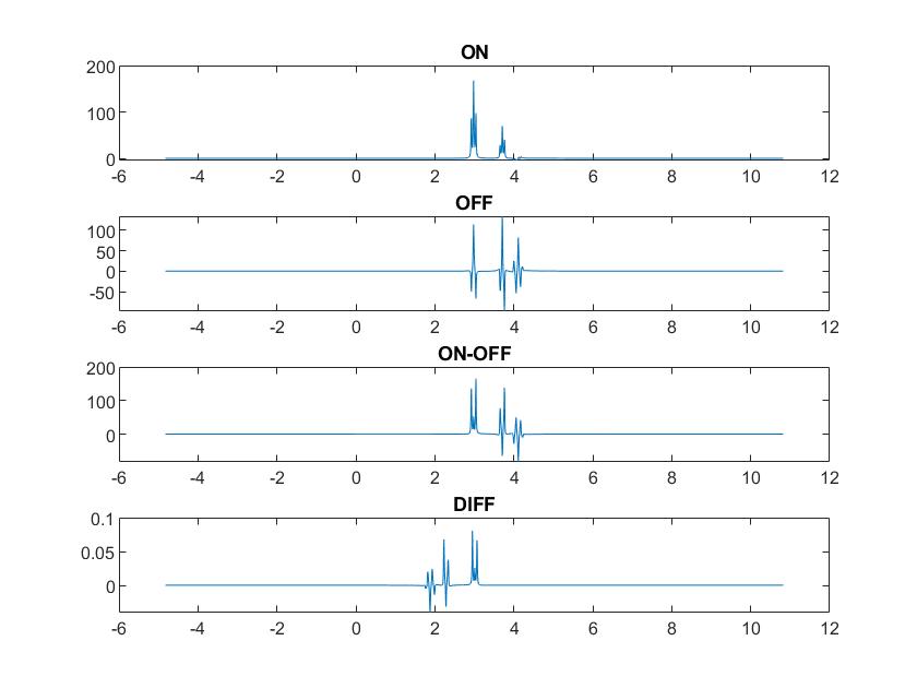
I have extracted the waveforms and timings from our GE MEGA-PRESS sequence and can now run a modified version of the run_sim_MegaPressShaped_fast.m script to create the ON, OFF and DIFF structures. The results look a bit odd though and I suspect that there is some bug in the script, since I get the same odd results also in running the original script. The ON and OFF spectra seems to be stored in the reverse direction, see image below. If I plot the ON.specs and OFF.specs in the reverse direction, i.e. (end:-1:1), I get the correct position of the spectral peaks. I have tried to look at the code but I can not find where it can go wrong, maybe you can help in debugging this. The DIFF spectra seem to be correctly stored but I don’t understand the change in scale (note the difference in y-scale for subplots 3 and 4).
Now that I can simulate the individual spectra I also need some help in how to package them into the .mat files that is read in the creation of the basis set (fit_makeBasis). What should be contained in the .mat files for the individual simulated spectra? I guess that it should be the ON, OFF and DIFF structures but should they be named in some specific way? Should the .mat file also be named in some specific way, e.g. ‘GABA’, ‘Lac’ and so fourth?
Cheers,
/Greger
Hi Greger,
Looks great at first sight, except for the inverted ppm axis indeed! I’m curious why the ON-OFF and the DIFF are different. How do you produce these two? And what’s the code you’re using to plot the data? If you like, feel free to share here (or upload to a GitHub repo and point to it), so I can take a look.
The units suggest that something about the order of the fft is a bit messed up. FID-A uses ifft to go from time domain to frequency domain and fft to return, and I believe ifft includes a division by the number of points, so spectral power isn’t maintained on a full cycle (I always thought it more intuitively the other way around, and have - regrettably - programmed all Osprey functions to go with my intuition rather than the FID-A convention). Flipping ifft and fft will likely do the trick, I’m just not entirely sure where in your code that needs doing.
Finally, I’ve worked on some instructions for importing FID-A simulations into an Osprey basis set. Hope to upload it by the weekend.
Let me know if that helps.
Best,
Georg
Hi Georg,
The code is simple enough. First of all I checked that I was using the original script.
>> which run_simMegaPressShaped_fast
C:\Users\greger.oradd\Downloads\FID-A-master\exampleRunScripts\run_simMegaPressShaped_fast.m
>> info=dir(‘C:\Users\greger.oradd\Downloads\FID-A-master\exampleRunScripts\run_simMegaPressShaped_fast.m’)
*info = *
- struct with fields:*
-
name: 'run_simMegaPressShaped_fast.m'* -
folder: 'C:\Users\greger.oradd\Downloads\FID-A-master\exampleRunScripts'* -
date: '11-May-2020 10:22:49'* -
bytes: 20494* -
isdir: 0* - datenum: 7.3792e+05*
Then running the script.
[ooutDIFF,ooutOFF,ooutON]=run_simMegaPressShaped_fast(‘GABA’);
Then I verified that the difference between DIFF and the other two is really in specs and not in ppm.
>> sum(ooutON.ppm-ooutOFF.ppm)
ans = 0
>> sum(ooutON.ppm-ooutDIFF.ppm)
ans = 0
And plotting it
figure(10)
subplot(4,1,1)
plot(ooutON.ppm,real(ooutON.specs))
title(‘ON’)
subplot(4,1,2)
plot(ooutOFF.ppm,real(ooutOFF.specs))
title(‘OFF’)
subplot(4,1,3)
plot(ooutON.ppm,real(ooutON.specs-ooutOFF.specs))
title(‘ON-OFF’)
subplot(4,1,4)
plot(ooutDIFF.ppm,real(ooutDIFF.specs))
title(‘DIFF’)
So the only code I have been using is actually from the FID-A script. The formation of the DIFF specs actually involves an ifft (in op_subtractScans.m) so you might be right in the guess that the scaling has something to do with fft/ifft but I’ll leave it up to you to verify and find the best workaround.
As for the reversed direction of the specs I have no clue to how the DIFF can be different from the ON/OFF. As far as I understand it DIFF is formed by op_subtractScans(outON,outOFF).
Hope that this helps,
/Greger
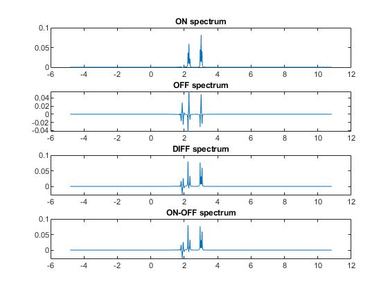
Hi again,
I found out what was going wrong in my simulations. I had put the Osprey paths above the FID-A paths so some op_ scripts were read from the Osprey paths and some from the FID-A paths. Hence the mix in fft/ifft use.
I put the FID-A path above Osprey and then it looks a bit more consistent.
I understand now that one really have to be careful not to mix the two packages, since many functions have the same name.
Now I’m looking forward to your instructions on how to create a basis set in Osprey.
Cheers,
/Greger
1 Like
Hi Greger,
Excellent, that would have been my next suggestion - the modified Osprey versions of the FID-A functions shadow the actual FID-A functions. In hindsight, I wish I hadn’t gone down that route… Might be something for a larger update in the future.
I’ll let you know here when I have added the documentation. Thanks for your time, I’m really delighted you’re digging into Osprey at this early stage of development.
Best wishes, and have a great weekend,
Georg