As an MRS user who use both OSPREY and GANNET, I know there’re some differences in their data analysis methods but unfortunately, I am recently encountering certain inconsistencies while analyzing the same MEGA-PRESS dataset.
The pattern that emerge after applying Gannet (such as the mean GABA_conc_Cr in patient group (0.103± 0.008) < normal group 0. 0.110± 0.006) differ from the patterns observed after using Osprey (where the mean GABAPlus scaled in Cr in patient group (0.324±0.051) > nomal group (0.284±0.055)). The data collection is ongoing and each group consists of only about 10 individuals, but these inconsistencies are causing me some concern.
Another thought is that maybe the current sample size is relatively small, so I shoundn’t be too worried?
For both methods, I ensured that the spectral alignment was set to RobSpecReg, and in Osprey, the opts.fit.coMM3 option was set to 3to2MM. I would greatly appreciate your advice on how to interpret these contrary results.
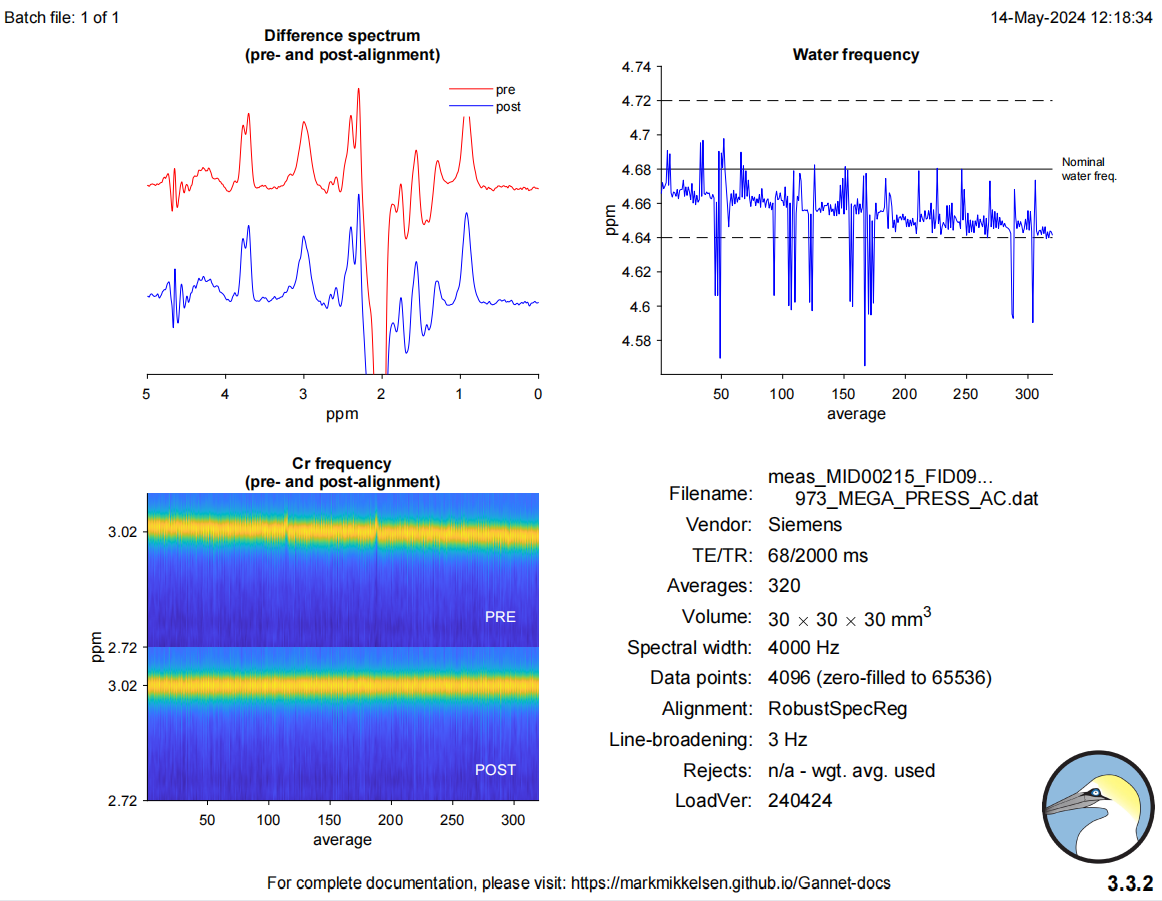
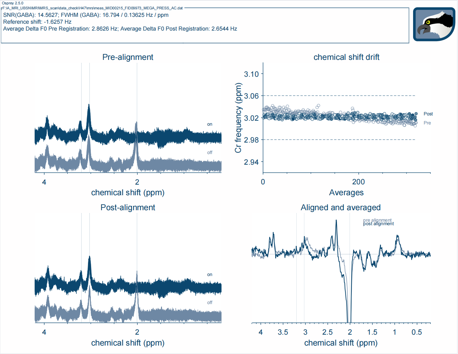
Additionally, I noticed that when assessing processing quality, the fluctuation in Cr frequency observed in Osprey appeared to be minimal, whereas in Gannet, the variation in water frequency seemed to be unacceptable. I uploaded two screenshot to show it.
Does this imply that Gannet employs a more stringent artifact removal procedure?
Your advice would be greatly appreciated! Thank you very much!
It’s not unusual for the outcomes to differ a bit (including broad differences of scale), but it really shouldn’t be changing the direction of your effect at this sample size! You’re right to be slightly concerned, but the data you show looks decent so this should be resolvable.
Firstly, did you filter for any outliers or other quality issues?
The water frequency estimation (top right of the figure) is a fairly crude first approximation – I believe it just looks for the most intense point in the frequency-domain spectrum near water. In some situations (eg, strong water suppression which doesn’t leave much residual water) it can be a bit less reliable, which is one reason to prefer other methods to fine-tune the alignment/registration. In the bottom left of that same figure, you can see the Creatine peak has been aligned quite well: note that the gradual drift and glitches around average 120 and 180 have been resolved, same as in the Osprey case.
No; the Robust Spectral Registration should be fairly similar in each; outliers are downweighted rather than removed outright.
The registration looks like it has worked correctly in both cases. However, the shape of some of the peaks looks a little peculiar – not terrible, but there might be an issue with phasing and I guess it might be more severe for some subjects. Did you acquire water-unsuppressed reference data too? If so:
Are you using this for eddy-current correction (ECC)?
Do you see similar effects in the water-referenced concentration estimates?
Could you please share images of the fitting outcomes, eg, the GannetFit output and the equivalent from Osprey (Overview or Fit) showing both the edited (DIFF, A) and edit-OFF sub-spectra?
Your explanation greatly helped me understand how to interpret the frequency estimation plots.
Firstly, did you filter for any outliers or other quality issues?
I didn’t filter any outliers, and actually I don’t know where osprey saved the outliers. I noticed that Gannet provides information on MRS_struct.out.reject for this purpose, but I couldn’t find a similar feature in Osprey.
Are you using this for eddy-current correction (ECC)?
Yes. We acquired water-unsuppressed data for each subject and used it as the reference.
Do you see similar effects in the water-referenced concentration estimates?
Yes. Tonight, I compared the GABA_conc_iu and GABA_ConcIU_CSFcorr from Gannet, the values from healthy group are always bigger than those in the patient group. However, Osprey shows the opposite trend.
I have uploaded the GannetFit and OspreyFit for both groups. Unfortunately, I’m unable to add text to annotate the PDFs, but I hope the current layout won’t hinder to review them.
Many thanks for your help. Your professionalism and kindness are greatly appreciated.
Could you also share the GannetLoad and OspreyProcess PDFs of these subjects?
Note that the default option in Gannet is to use weighted averaging. Outliers are not removed; instead, averages determined to be of lower quality than the rest of the averages are down-weighted (see more here).
Thanks for uploading the figures. At first glance, your GannetFit output looks good – I don’t notice any issues there.
By contrast, several of the fits from Osprey for the edited (difference) spectrum seem problematic – notice quite substantial signals in the residuals (top part of the output plot) and a wildly fluctuating baseline (thin blue curve underlying the yellow fit). Several of your spectra have quite strong and strangely shaped signals to the right of the negative NAA peak (around 1.6 ppm), but I don’t think that’s the only issue. Gannet may be better at detecting (and filtering) fluctuating signal in that region, and in any case it’s outside the main fit range for that algorithm.
Perhaps @Helge has some more concrete suggestions for improving the Osprey fit? It may help if you could share details of the Osprey configuration you used (eg, your Osprey job file).
Extra-long weekend here , so I may not be able to follow up in detail until mid next week.
I agree with Alex, and I would be particularly curious to see the PDF protocol of the scan. This is the CMRR sequence, yes? I’m not super-sure that we know how the editing pulse is shaped in that one, and the specified duration/bandwidth is not unlikely to not be accurately reflected in the simulations for the basis set (the poor fit to both Glx signals gives it away).
Thanks for offering the time to help and review the documents.
I have uploaded all the Osprey_process/Gannet_load, the PDF protocol of the scan, as well as the configured Osprey Job file (revised a little bit at the end to save the files to designated destination).
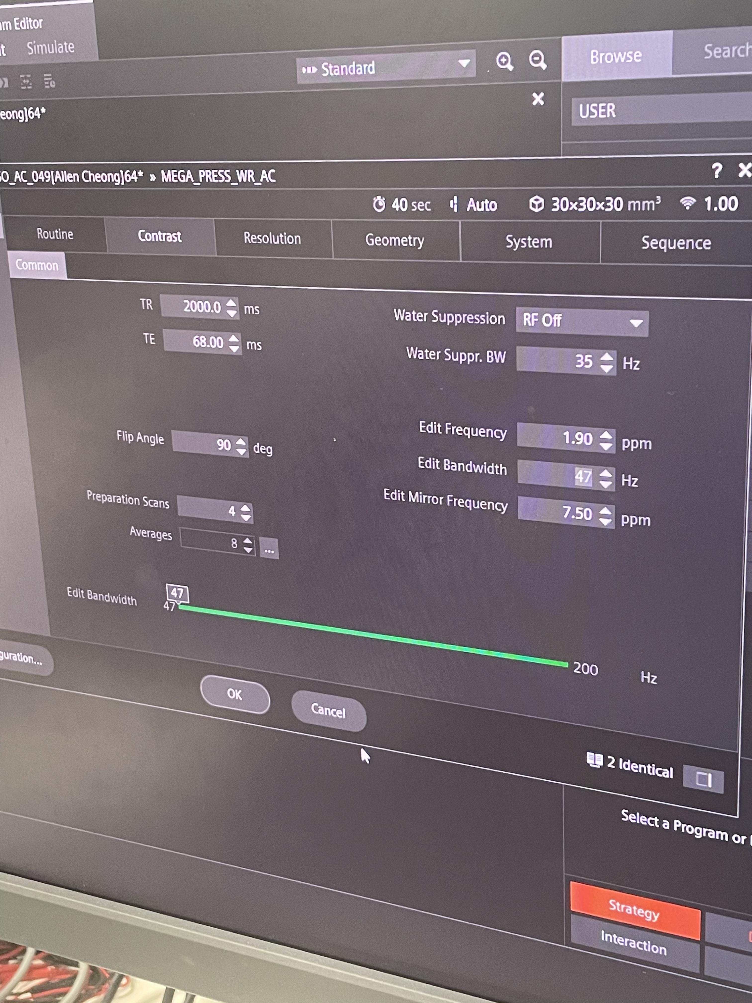
The editing pulse bandwidth value in the protocol trips me up a little. It doesn’t help that this is the MEGA product sequence on XA30 and I do not know the details very well.
I know that the Siemens MEGA sequences generally use a weirdly filtered editing pulse (there is no way that a truly 47-Hz FWHM Gaussian-ish pulse fits in the gaps of TE68 PRESS localization module). Is 47 Hz the lowest value that you were able to select?
I’m going to have to do some digging to figure out what duration/“true” bandwidth this pulse has. @wclarke do you have access to the XA30 MEGA-PRESS by any chance?
Thanks for the quick feedback. As I can remember the 47
Hz indeed is the lowest bandwidth value we can select where I took your suggestion from a previous post. I’ll double confirm it from the MRI center tmr. The default protocol that we had from Siemens was set it to 70Hz.
Hope the current MEGA PRESS sequence is not too bad.
I believe this is product now. 47 Hz * 1.37 = 64.4 Hz still strikes me as too low an attainable bandwidth for TE = 68 ms. If the pulses are still the same as in the old WIP that Thomas’ paper refers to (with an estimated time-(actual)-bandwidth product of 25.6 * 1e-3 s * 48.2 Hz = 1.232), that bandwidth would require a 20-ms pulse. With 2.6-ms excitation and 5.2-ms refocusing pulses (assuming this is still the same PRESS backbone it’s always been), that leaves very little room for gradients.
I seem to remember that Thomas also found that the editing pulse waveform wasn’t actually sinc-Gaussian - I believe I have his code somewhere but would need to dig deeper, but I would also be surprised if they hadn’t fixed the pulse in the meantime. (Or maybe I wouldn’t)
@Melinna The reason why all this matters is that the editing pulse bandwidth determines the shape of the co-edited metabolite signals (for MEGA-PRESS, that will be most notably NAA and Glx, which doesn’t seem to be modeled correctly in your data) as well as the co-edited macromolecular signals. GABA itself will not be directly affected since the editing pulse center is set to its 1.9-ppm protons, no matter how broad the pulse is (there are secondary effects caused by drift, but they’re probably negligible here). I’ll try to gather more information about this sequence but since we don’t have it ourselves this may well take a while.