How to do manual integration to quantify metabolite concentration?

[zui]

Hi,

Suppose there is a spectrum with only two peaks, but the two peaks are close to each other, and one of them is more than 10 times larger the other peak.

I intend to follow these steps to quantify the amount of metabolites:

1. zero order and first order phase correction
2. estimate the linewidth (FWHM) of the two peaks
3. Integrate the real part of each peak with the same integral range 2*max([FWHM_peak1,FWHM_peak2]) and centered at the resonance frequency of each peak

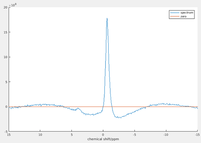
However, after phase correction, the spectrum now looks like this

If I simply integrate the real part, then the result for the higher peak will be positive but that of the lower peak will be a negative value!

What should I do? Or, in this case, it’s generally not recommended to use “manual integration” method?

Thanks for your advice!

[ChiaHsu]

Hello,

The procedure you’ve described sounds like what organic chemists typically do when manually analyzing their NMR spectra (peak picking, integration, and multiplet analysis). They commonly use software like Bruker TopSpin (free) and MestReNova, which offer sophisticated tools for phasing, baseline correction, and peak integration. There are many video tutorials available for these NMR processing software packages.

While manual integration can work well for NMR spectra, the situation you’ve described is particularly challenging. The negative integration value for your smaller peak suggests significant baseline distortion, which is common in X-nuclei MRS acquired on MRI scanners due to their much longer deadtimes compared to dedicated NMR spectrometers. A proper phasing will be very challenging, too, and you will need to do good baseline correction after a proper phasing.

Since we previously discussed using AMARES (OXSA) for time-domain fitting that circumvents the phasing problem, I’m just curious—is there specific information you’re trying to obtain that isn’t accessible through OXSA?

Thanks!

[zui]

Thank you! I’m surprised that you still remember our discussion last time.

@ChiaHsu

They commonly use software like Bruker TopSpin (free) and MestReNova

We have Bruker Topspin, but the spectra were not acquired with a Bruker scanner, and I find it challenging to import the datasets into Bruker Topspin.
It’s my first time to hear MestReNova.

@ChiaHsu

A proper phasing will be very challenging, too, and you will need to do good baseline correction after a proper phasing.

For phase correction, we simply used first order phase correction, i.e., set beginTime equal to TE, and manually twist the zero order phase correction angle until all peaks point upwards.

I’m very curious what a good baseline should look like and how to get such a baseline.

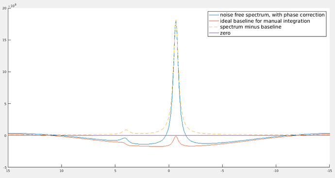
After I raised this question in the forum, I tried on my own and discovered that, an ideal baseline should look like this

The blue spectrum is a simulated one. The yellow dashed line represents the spectrum when the two peaks both have zero phase angle.

@ChiaHsu

Since we previously discussed using AMARES (OXSA) for time-domain fitting that circumvents the phasing problem, I’m just curious—is there specific information you’re trying to obtain that isn’t accessible through OXSA?

Yes, this is still the same hyperpolarized 13C spectra of a rat liver as in our previous discussion.

OXSA and AMARES performs well for some rats/time frames, but not very well for some other rats/time frames. I’ve tried very hard to adjust the prior knowledge but it happens quite often that when there is clearly no signal of Leucine peak, AMARES reports there is some signal, or when there is a small signal but AMARES reports there is a big signal.

Actually all I want is just an accurate estimate of relative signal strength of matabolites. Because of the noise and some other confounding factors, AMARES doesn’t seem robust enough. That’s why I thought about integration.

[ChiaHsu]

I understand that adjusting prior knowledge for AMARES is cumbersome. However, on the other hand, manual baseline correction is quite subjective, and automatic baseline correction algorithms (e.g. polynomial or Whittaker smoother) still need you to adjust smoothing parameters to make them visibly work well. Thus, the accuracy of the peak integration method depends heavily on the robustness of baseline correction (and phasing).

Btw, why does your simulated “ideal baseline for manual integration” still have two visible peaks? Usually, we would like the baseline-corrected spectrum to have flat baselines. This is a “fully automatic baseline correction” paper from MestReNova, just fyi (Redirecting ). The algorithm is very robust and is validated on the rolling baseline of a 13C NMR with a long pre-acquisition delay (somewhat similar to a 13C MRS). However, it still has two parameters to be tuned according to your specific scenario.

In addition to this one, there are also many other baseline correction algorithms available, including more recent deep-learning approaches - I hope you can find one that fits your needs.

[zui]

Hi!
I really admire your efficiency in searching for papers!

@ChiaHsu

why does your simulated “ideal baseline for manual integration” still have two visible peaks?

The “noise free spectrum, with phase correction” has first order phase correction. The “spectrum minus baseline” doesn’t have first order phase correction (its effect has been removed by subtracting the baseline.) The two smaller peaks are to correct the dispersion part that goes into the real part of the spectrum because of first order phase correction.

@ChiaHsu

Usually, we would like the baseline-corrected spectrum to have flat baselines.

Yes, it does look much smoother if you zoom out. It becomes so unnatural because the visible ppm range is so small. As you can see, the bump of the smaller peak looks “flatter and smoother” than that of the higher peak. However, if you zoom in to the region near that smaller peak, its bump will look more obvious.

The small bump can be understood in this intuitive way: suppose the higher peak is at 172.6 ppm. After first order phase correction, the point at 172.6 ppm on the spectrum will be exactly in phase (i.e., the imaginary part is zero, the real part is equal to the magnitude). To the left of 172.6 ppm, it’s a bit off phase, and to the right, it’s a bit off phase to the other direction. Because at the point of 172.6 ppm, it’s exactly in phase, so we don’t need to correct anything for that point, i.e., baseline at 172.6 ppm should be equal to zero. Then there must be such a bump.

@ChiaHsu

manual baseline correction is quite subjective, and automatic baseline correction algorithms (e.g. polynomial or Whittaker smoother) still need you to adjust smoothing parameters to make them visibly work well.

Yeah, I’m now looking through the spectra one by one (over 700 spectra to go through) and adjusting the polynomial for every spectrum… That being said, for some spectra with low SNR, the error is quite large (about 25%) even when two baselines look identical.

@ChiaHsu

there are also many other baseline correction algorithms available, including more recent deep-learning approaches - I hope you can find one that fits your needs.

Sadly, it might be my inadequate understanding of papers. In my past experience, it happened quite a few times when I spent some time reading papers and implementing the algorithm or learning how to use their package only to find that it doesn’t work as well as expected.
By the way, does anyone share similar experiences? I don’t mean the methods in those papers are not good. Just feel that there is the risk not to get expected result after trying new (even classic, sometimes) algorithms.
And when two methods happen to work reasonably well but the results differ… Then there must be something wrong. But I don’t know what is wrong. Then I would begin to doubt “what on earth that I know is truly true?”
Anyways, I don’t have the time to try out other methods as I need to finalize the results by today. I raised this question in the beginning because I was doubting whether a polynomial can mimick an ideal baseline. It seems that the difference is just the area of that small bump. With low SNR, I guess it’s negligible.

Thank you!!