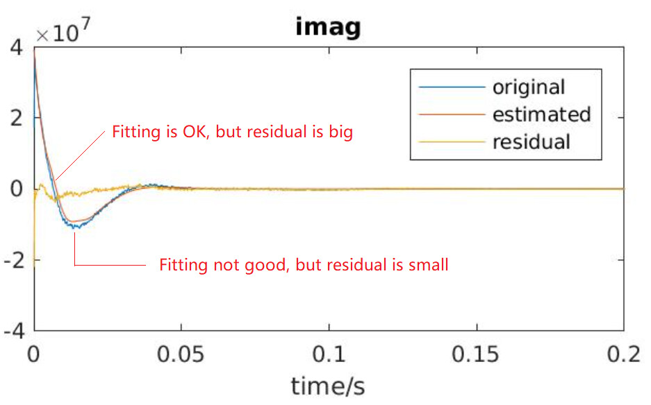
As I was trying with AMARES in OXSA, my fitting result is always bad (fit quality number, FQN, is around 6). And I noticed this strange behaviour, as shown in the graph. I guess AMARES (essentially a non-linear least square fitting algorithm) tries very hard to minimize the residual of the steep part and as a consequence, omits the resdisual of the relatively gentle part.
I wanted to improve the fitting by applying smaller weight to the steep part and larger weight to the gentle part. Is it possible to do this in OXSA? Or do I have to modify its source code?
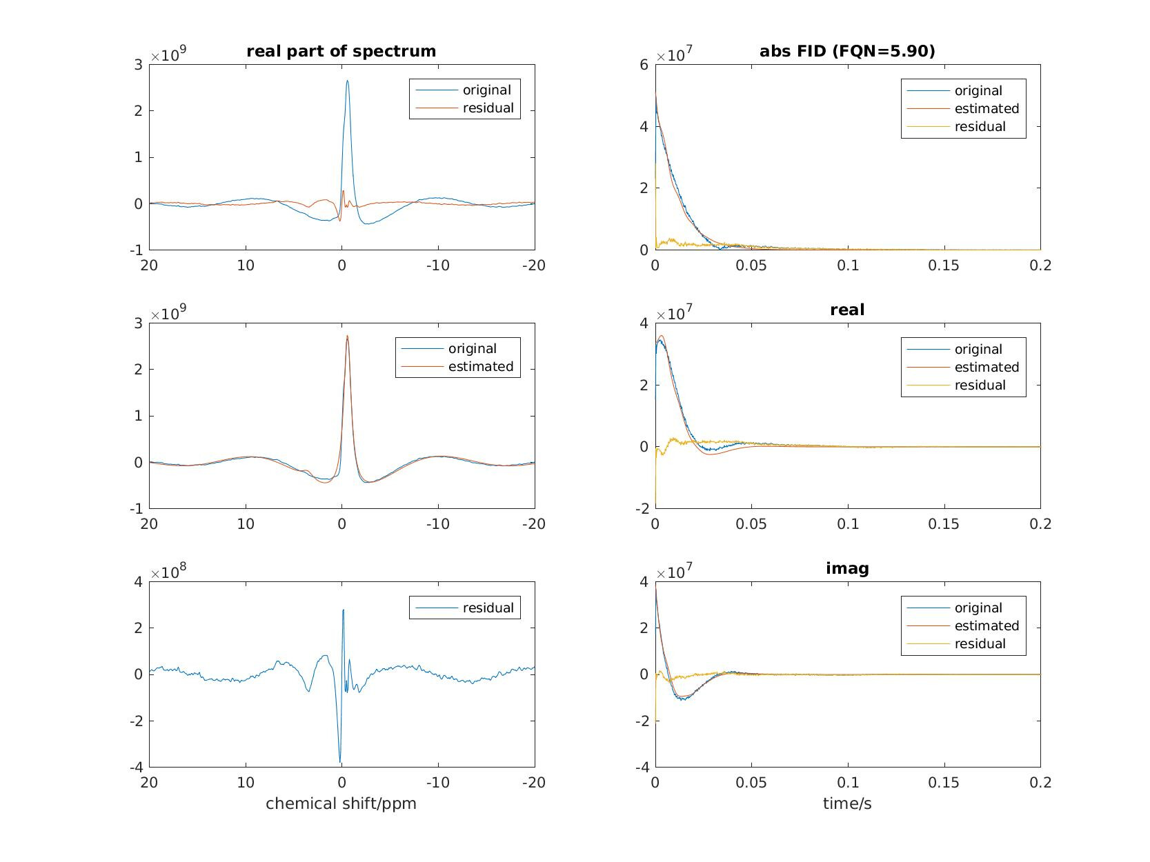
What do the data (and the model) look like in the frequency domain? It’ll be easier to judge failure or success if we can actually see the peaks you’re trying to model.
One thing I’m noticing here is the first point in the data, which appears to be lower than the top of the echo - are you sure the receiver was turned on at the correct time? You might consider cropping that point (which will also help the model)
PyAMARES supports user-defined objective functions for minimization, making it quite flexible. For example, you can fit selected parts of the FID (frequency-selective AMARES). Weighing the FID is also technically feasible to implement in the objective function.
However, it seems what you’re looking for might be achieved by applying Gaussian or Sine Bell apodization to the FID before AMARES fitting, which wouldn’t require modification of the source code of OXSA, or defining your own objective function in pyAMARES.
If your large peak is on-resonance and the smaller peak is off-resonance, it appears you’re trying to down-weight the large peak while somehow up-weighting the smaller one.
I agree with the admin that cropping the first point(s) could be helpful. You will just need to adjust the dead time (beginTime in OXSA) accordingly.
However, it is hard to discuss the AMARES fitting without context, as prior knowledge is critical for AMARES fitting. If possible, could you provide more context about your prior knowledge? Are these two singlets? Do you have any constraints on the phase, frequency, amplitude, linewidths, or lineshape? Are they pure Lorentzian, Gaussian, or Voigt?
Thanks for your insight. I also noticed the first point of FID looks strange but I never thought about why. I fed the original fid to amaresFit in OXSA without any preprocessing (of course I have edited the prior knowledge file)
are you sure the receiver was turned on at the correct time
I don’t know. The raw data were collected by our collaborators.
Below is some more information about the fit result and prior knowledge.
I don’t know. I treat them as singlets in the prior knowledge though.
Are they pure Lorentzian, Gaussian, or Voigt?
I never tried with other lineshapes, except Lorentzian. Maybe I can open a new topic to ask “When is it appropriate to use line shapes other than a pure Lorentzian”
I’ll have a try. Thanks for the suggestion.
I know Gaussian, Lorentzian, and Lorentzian-to-Gaussian apodization, and roughly know their effect in time domain and frequency domain. But it’s my first time to hear Sine Bell apodization. May you explain why you think Gaussian or Sine Bell apodization is likely to solve the problem? (Maybe you thought that way because I hadn’t shown what the signal looks like in frequency domain)
Lorentzian lineshape usually works well unless it is proven that Lorentzian renders a poor fit.
As I mentioned before, I only recommend apodization for visualization (better resolution/sensitivity of the FT’d spectrum). I brought up sine-bell apodization because it seems you want to de-emphasize the beginning part (“steep part”) of the FID. You can find different apodization methods in the book “NMR Data Processing” by Jeff Hoch, or check this Mestralab help page: (Apodization)
P.S. Could you check your fitted values (especially linewidth) against the constraints in your prior knowledge? You set 30-50 Hz for both the big and small peaks, which seems quite restrictive. And if I recall correctly, OXSA optimizes its initial conditions by varying amplitudes and phases only before doing the AMARES fitting. So be cautious when setting your initial chemical shifts and linewidths in the prior knowledge dataset. You may want to fine-tune these initial values (and sometimes constraints) to get a good fit.
Thanks for the hint on linewidth. I just noticed that the estimated linewidth for Leucine is 49.99, reaching the bound of linewidth [30,50].
Initially I set both linewidths to [30,50] because the values are within this interval for those good fit (FQN is around 1). I assume if it’s the same rat, the same position in the scanner, the same sequence, …, everything identical, except that some data are acquired earlier than others, then the linewidth (essentially the T2*) would also be within this interval. Is it normal to see linewidth of the same peak changes over 30 Hz when all acquisition parameters are identical?
I should examine my prior knowledge again, especially those whose estimated values have reached the bound.
If all parameters are identical, a variation of over 30 Hz seems unusually large. However, I can’t be certain, as the linewidth can be significantly affected by shimming or animal motion.