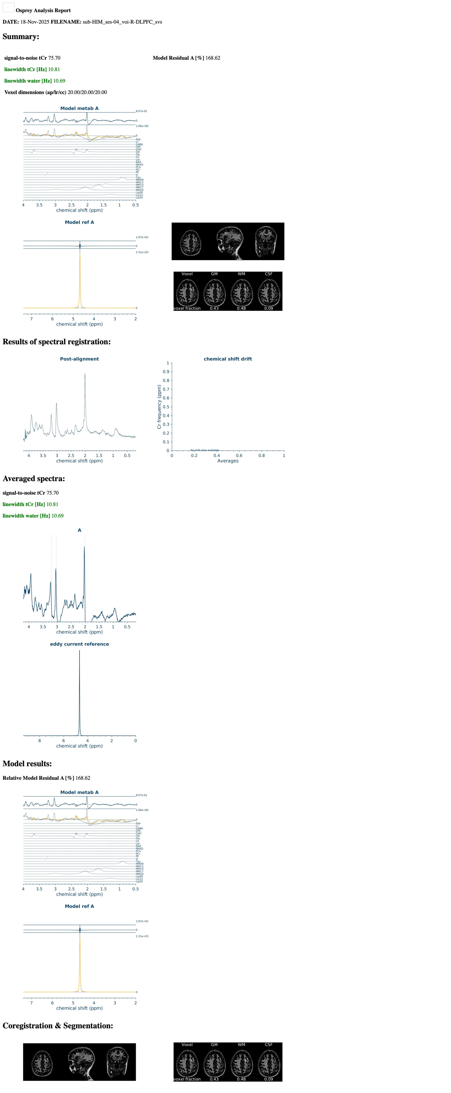
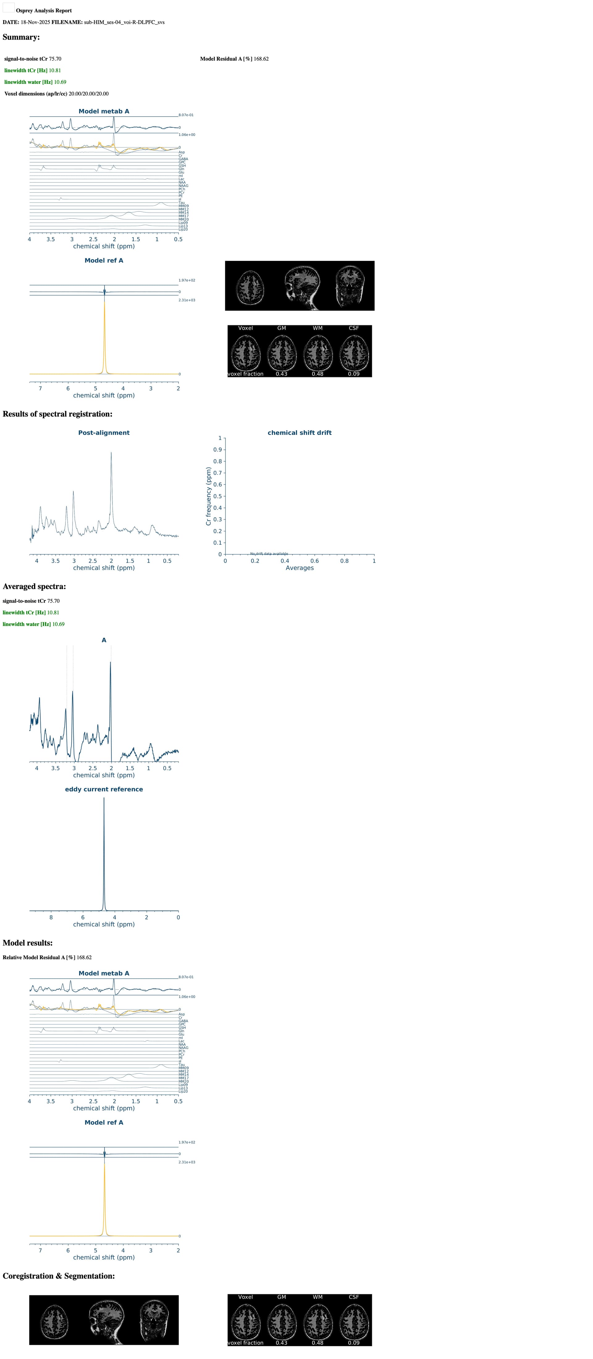
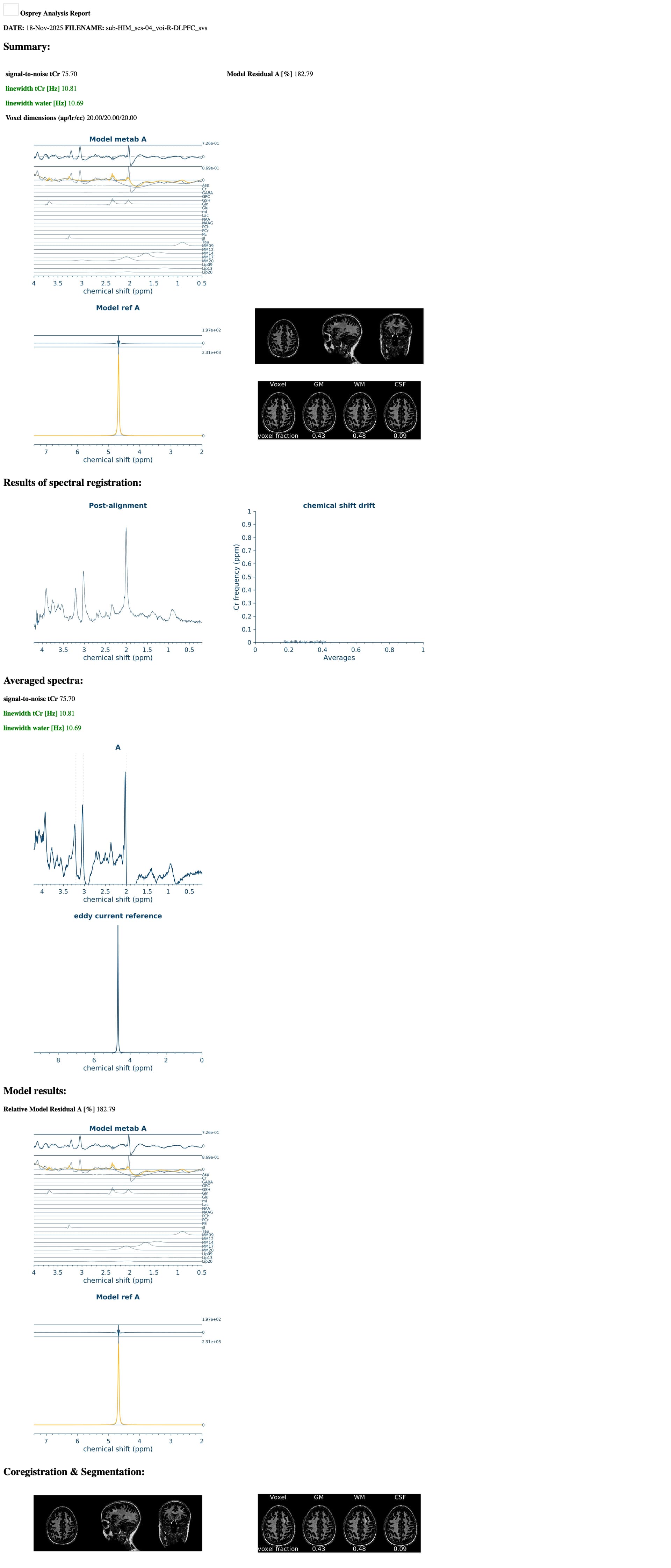
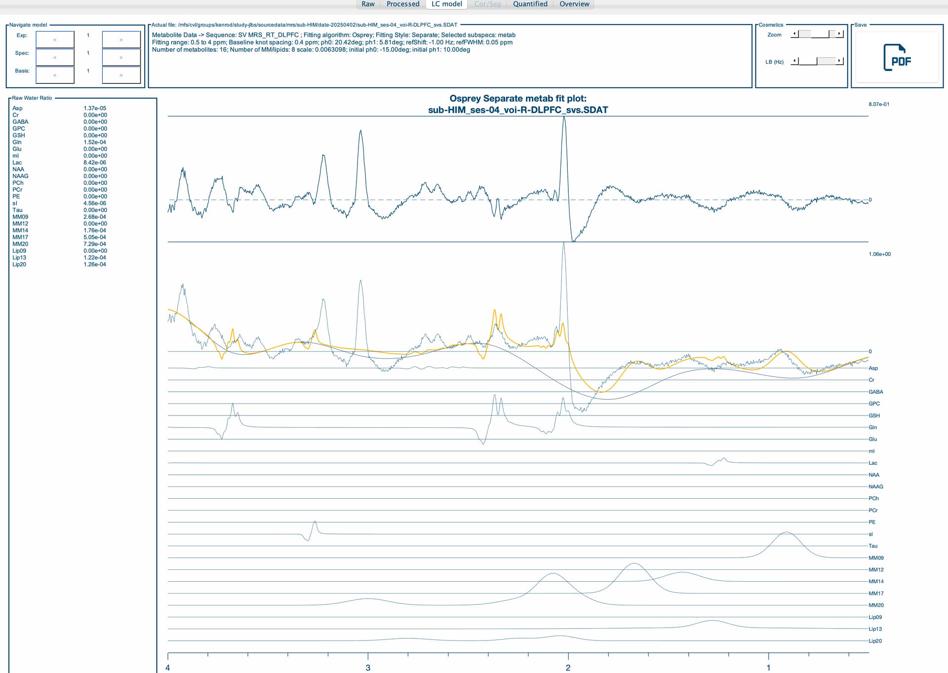
I am running an Osprey job file and I am getting different metabolite quantifications depending on which computing node I am running them on. I am running the exact same job file, including the same basis set, T1 and water reference. It appears to be at the coregister step, specifically the results of MRSCont.fit.results.metab.fitParams{1,1} results seem to differ across nodes. Do you have any idea as to why this may be? It will not allow me to attach the .mat files, but I have attached the report which shows differences in the upper and lower bounds on the fit residuals between nodes. Any help you can provide would be greatly appreciated!
Edit: I will have to do them one at a time. I get the following error message when trying to get help with an Osprey error
An error occurred: Sorry, new users can only put one embedded media item in a post
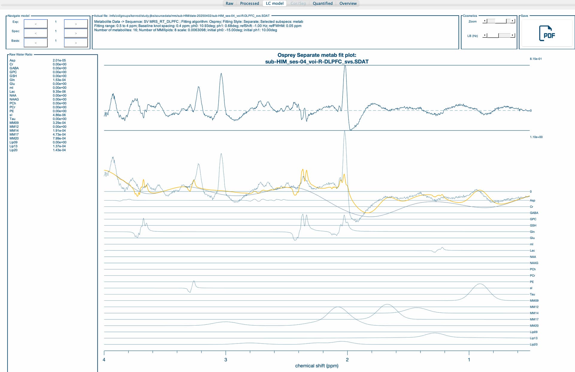
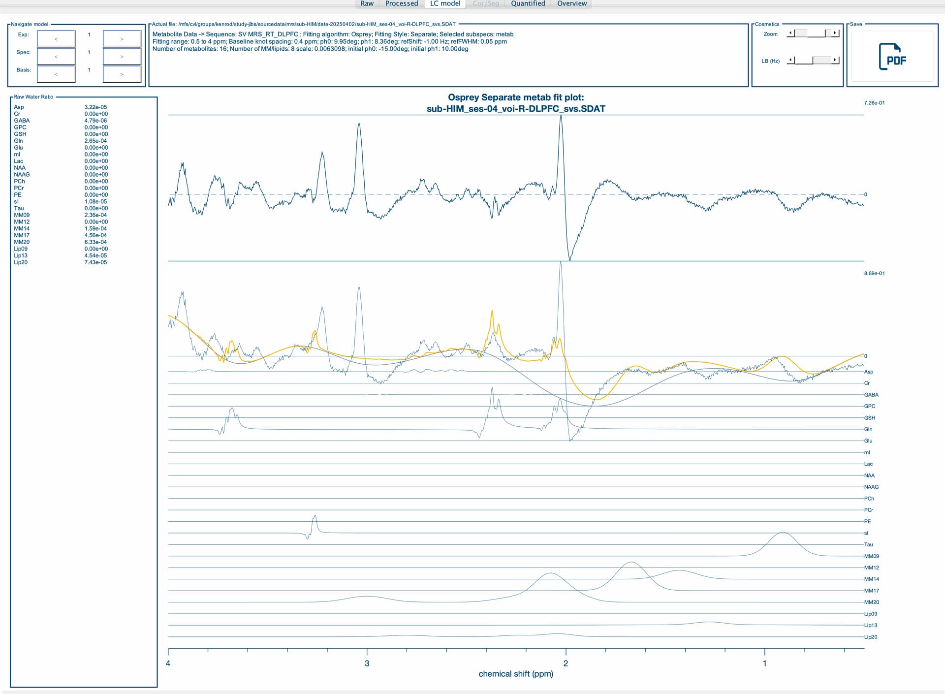
Thank you so much for your quick reply! Of course, I have attached the OspreyFit and Quantify Results for each node. Compute-04 and compute-16 seem to be similar, so I’ve included all the information for nodes compute-02, compute-05 and compute-16 (we have roughly another 5 nodes and can’t always control what nodes they get assigned to). Let me know if there is a different format you would like these in.
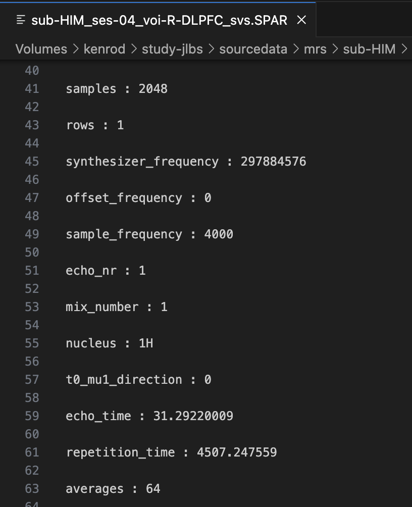
The first thing to note is that the wrong basis set is being used. I suspect is that your MRS data were acquired at long TE (e.g., TE = 120 ms). Is that right? Also, the phasing is off, but that might be due to the fitting procedure.
I’m not sure why you’re getting different fitting results each time the data are fit, though. Could you explain why each node is running on the same dataset?
My apologies for the delay. In regards to the basis set, we have an existing .BASIS that I converted using the io_LCMBasis command. I believe I used the correct flags, however, if there is an apparent error, please let me know (I have some knowledge of MRS processing and quantification, but am a novice when it comes to the physics and basis set side of things).
I am attaching our exam card for the MRS scan (.txt file attached) . Our MR Tech recommended that we use the “shortest” TR/TE on the 7T Philips scanner, and has provided us a basis set with TE=30. In the pilot scan above, this equates to a TE=31.29 ms, which she has stated makes a negligible difference.
Regarding running the same participant on different nodes, we were doing this for testing purposes to create a pipeline for our study, and noticed that we are getting vastly different quantifications, even though we are using the exact same job file (including same voxel (R-DLPFC), same water reference and same basis set and getting different results). I am puzzled as to these differential findings.
We’re unfortunately aware of (mostly subtle) differences depending on the computational environment. That is really regrettable - it boils down to some of the Osprey processing and fitting routines using numerical gradient calculations, and those appear to vary between machines. This will be a problem of the past once we release Osprey 3 (which uses all analytical gradient calculations) - hopefully within a few weeks, we’re testing and writing documentation.
It is correct that the fit is a complete failure, likely because the basis set conversion didn’t work as intended. Instead of trying to convert the LCModel basis set back to Osprey, I suggest that you let Osprey pass the fitting off to LCModel instead. That way, you can just use the basis set as is. It should also take care of any computational differences between nodes (fingers crossed).
For that, work from this job file template. Specifically, besides the other things you modify, check these settings:
%%% ----- LCMODEL FITTING OPTIONS -----
% Specify LCModel-format basis set (.BASIS)
% If no basis set file is provided Osprey will generate the .BASIS file
% from Ospreys database
% opts.fit.basisSetFile       = {which('3T_press_Philips_35ms_noMM.BASIS')};


% Specify LCModel-type control file (.CONTROL)
% This is optional: If you leave this field blank, Osprey will create a
% minimum control file for you.
% opts.fit.controlFile        = '';


% Specify custom LCModel binary path
% You can set the path to a custom-compiled LCModel binary here. If left
% empty, Osprey will try to use one of the pre-compiled binaries it is
% shipped with.
% opts.fit.customLCModelBinary = 'C:\Users\goeltzs1\Documents\MATLAB\osprey\libraries\LCModel\custom\LCModel.exe';
%%% ----- END LCMODEL FITTING OPTIONS -----
Here, you can:
specify the full path to the .BASIS file in opts.fit.basisSetFile
if you want to let Osprey build a suitable LCModel control file, you can leave the opts.fit.controlFile commented out; otherwise, you can provide the path to a control file template with any additional settings you want to pass
finally, depending on the computational environment of the cluster, Osprey will already have a Unix-based LCModel executable built-in. If it doesn’t work, it’ll throw an error, and we’ll need to compile an executable that is suitable for that cluster (instructions here), and then point to the path of that executable. I can help with that if needed.
Thank you so much for the recommendation of passing the fitting off to LCModel. Using the original .BASIS file works perfectly, and drastically reduced the variance of quantification between nodes down to a fraction of a percent. Thank you both so much for your help in resolving this!
Interesting to hear that they’re still not identical. I suppose there might be minute differences to the data themselves resulting from precision differences during the processing (e.g. spectral registration). But glad to hear it appears at least much, much smaller.