%% jobSDAT.m
% This function describes an Osprey job defined in a MATLAB script.
%
% A valid Osprey job contains four distinct classes of items:
% 1. basic information on the MRS sequence used
% 2. several settings for data handling and modeling
% 3. a list of MRS (and, optionally, structural imaging) data files
% to be loaded
% 4. an output folder to store the results and exported files
%
% The list of MRS and structural imaging files is provided in the form of
% cell arrays. They can simply be provided explicitly, or from a more
% complex script that automatically determines file names from a given
% folder structure.
%
% Osprey distinguishes between four sets of data:
% - metabolite (water-suppressed) data
% (MANDATORY)
% Defined in cell array “files”
% - water reference data acquired with the SAME sequence as the
% metabolite data, just without water suppression RF pulses. This
% data is used to determine complex coil combination
% coefficients, and perform eddy current correction.
% (OPTIONAL)
% Defined in cell array “files_ref”
% - additional water data used for water-scaled quantification,
% usually from short-TE acquisitions due to reduced T2-weighting
% (OPTIONAL)
% Defined in cell array “files_w”
% - Structural image data used for co-registration and tissue class
% segmentation (usually a T1 MPRAGE). These files need to be
% provided in the NIfTI format (.nii) or, for GE data, as a
% folder containing DICOM Files (.dcm).
% (OPTIONAL)
% Defined in cell array “files_nii”
% - External segmentation results. These files need to be
% provided in the NIfTI format (*.nii or *.nii.gz).
% (OPTIONAL)
% Defined in cell array “files_seg” with 1 x 3 cell for each
% subject or 1 x 1 cell if a single 4D NIfTI is supplied.
%
% Files in the formats
% - .7 (GE)
% - .SDAT, .DATA/.LIST, .RAW/.SIN/.LAB (Philips)
% - .DAT (Siemens)
% - .nii, .nii.gz (NIfTI-MRS)
% usually contain all of the acquired data in a single file per scan. GE
% systems store water reference data in the same .7 file, so there is no
% need to specify it separately under files_ref.
%
% Files in the formats
% - .DCM (any)
% - .IMA, .RDA (Siemens)
% may contain separate files for each average. Instead of providing
% individual file names, please specify folders. Metabolite data, water
% reference data, and water data need to be located in separate folders.
%
% In the example script at hand the MATLAB functions strrep and which are
% used to generate a relative path, which allows you to run the examples
% on your machine directly. To set up your own Osprey job supply the
% specific locations as described above.
%
% AUTHOR:
% Dr. Georg Oeltzschner (Johns Hopkins University, 2019-07-15)
% goeltzs1@jhmi.edu
%
% HISTORY:
% 2019-07-15: First version of the code.
%%%%%%%%%%%%%%%%%%%%%%%%%%%%%%%%%%%%%%%
%%% 1. SPECIFY SEQUENCE INFORMATION %%%
% Specify sequence type
seqType = ‘unedited’; % OPTIONS: - ‘unedited’ (default)
% - ‘MEGA’
% - ‘HERMES’
% - ‘HERCULES’
% Specify editing targets
editTarget = {‘none’}; % OPTIONS: - {‘none’} (default if ‘unedited’)
% - {‘GABA’}, {‘GSH’}, {‘Lac’}, {‘PE322’}, {‘PE398’} (for ‘MEGA’)
% - {‘GABA’, ‘GSH’}, {‘GABA’, ‘Lac’}, {‘NAA’, ‘NAAG’} (for 'HERMES’and ‘HERCULES’)
% Specify data scenario
dataScenario = ‘invivo’; % OPTIONS: - ‘invivo’ (default)
% - ‘phantom’
% - ‘PRIAM’
% - ‘MRSI’
%%%%%%%%%%%%%%%%%%%%%%%%%%%%%%%%%%%%%%%
%%%%%%%%%%%%%%%%%%%%%%%%%%%%%%%%%%%%%%%%%%%%%%%%%%%%%
%%% 2. SPECIFY DATA HANDLING AND MODELING OPTIONS %%%
% Which spectral registration method should be used? Robust spectral
% registration is default, a frequency restricted spectral registration
% method is also availaible and is linked to the fit range.
opts.SpecReg = ‘RobSpecReg’; % OPTIONS: - ‘RobSpecReg’ (default) Spectral aligment with Water/Lipid removal, using simialrity meric, and weighted averaging
% - ‘ProbSpecReg’ Probabilistic spectral aligment to median target and weighted averaging
% - ‘RestrSpecReg’ Frequency restricted (fit range) spectral aligment, using simialrity meric, and weighted averaging
% - ‘none’
% Which algorithm do you want to align the sub spectra? L2 norm
% optimization is the default. This is only used for edited MRS!
% Which algorithm do you want to align the sub spectra? L2 norm
% optimization is the default. This is only used for edited MRS!
%Perform correction on the metabolite data (raw) or metabolite
%-nulled data (mm).
opts.SubSpecAlignment.mets = ‘L2Norm’; % OPTIONS: - ‘L2Norm’ (default)
% - ‘L1Norm’
% - ‘none’
%Perform eddy-current correction on the metabolite data (raw) or metabolite
%-nulled data (mm). This can either be done similar for all data sets by
%supplying a single value or specified for each dataset individually by supplying
% multiple entries (number has to match the number of datasets) e.g. to perform ECC
% for the second dataset only:
% opts.ECC.raw = [0 1];
% opts.ECC.mm = [0 1];
opts.ECC.raw = 0; % OPTIONS: - ‘1’ (default)
opts.ECC.mm = 0; % - ‘0’ (no)
% - array
% Save LCModel-exportable files for each spectrum?
opts.saveLCM = 1; % OPTIONS: - 0 (no, default)
% - 1 (yes)
% Save jMRUI-exportable files for each spectrum?
opts.savejMRUI = 0; % OPTIONS: - 0 (no, default)
% - 1 (yes)
% Save processed spectra in vendor-specific format (SDAT/SPAR, RDA, P)?
opts.saveVendor = 0; % OPTIONS: - 0 (no, default)
% - 1 (yes)
% Save processed spectra in NIfTI-MRS format?
opts.saveNII = 0; % OPTIONS: - 0 (no, default)
% - 1 (yes)
% Save PDF output for all Osprey modules and subjects?
opts.savePDF = 1; % OPTIONS: - 0 (no, default)
% - 1 (yes)
% Select the metabolites to be included in the basis set as a cell array,
% with entries separates by commas.
% With default Osprey basis sets, you can select the following metabolites:
% Ala, Asc, Asp, bHB, bHG, Cit, Cr, Cystat, CrCH2, EtOH, GABA, GPC, GSH, Glc, Gln,
% Glu, Gly, H2O, mI, Lac, NAA, NAAG, PCh, PCr, PE, Phenyl, sI, Ser,
% Tau, Tyros, MM09, MM12, MM14, MM17, MM20, Lip09, Lip13, Lip20.
% If you enter ‘default’, the basis set will include all of the above
% except for Ala, bHB, bHG, Cit, Cystat, EtOH, Glc, Gly, Phenyl, Ser, and Tyros.
opts.fit.includeMetabs = {‘Ala’, ‘Asp’, ‘Cr’, ‘GABA’, ‘Glc’, ‘Gln’, ‘Glu’, ‘GPC’, ‘GSH’, ‘Lac’, ‘mI’, ‘NAA’, ‘NAAG’, ‘PCh’, ‘PCr’, ‘sI’, ‘Tau’};
% OPTIONS: - {‘default’}
% - {custom}
% Choose the fitting algorithm
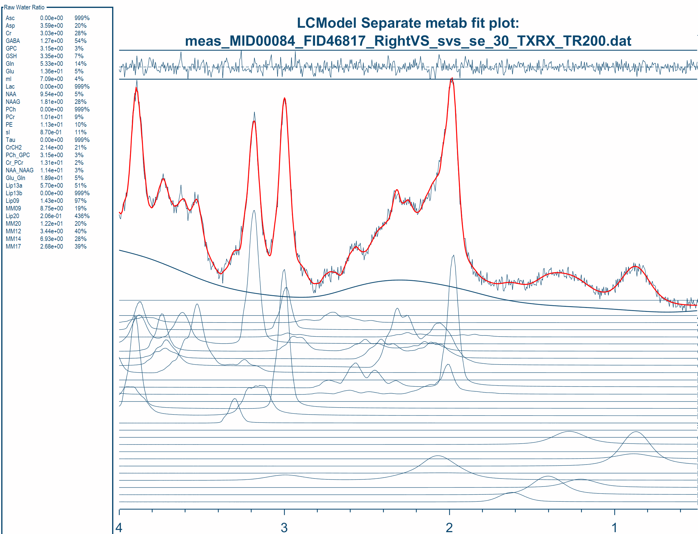
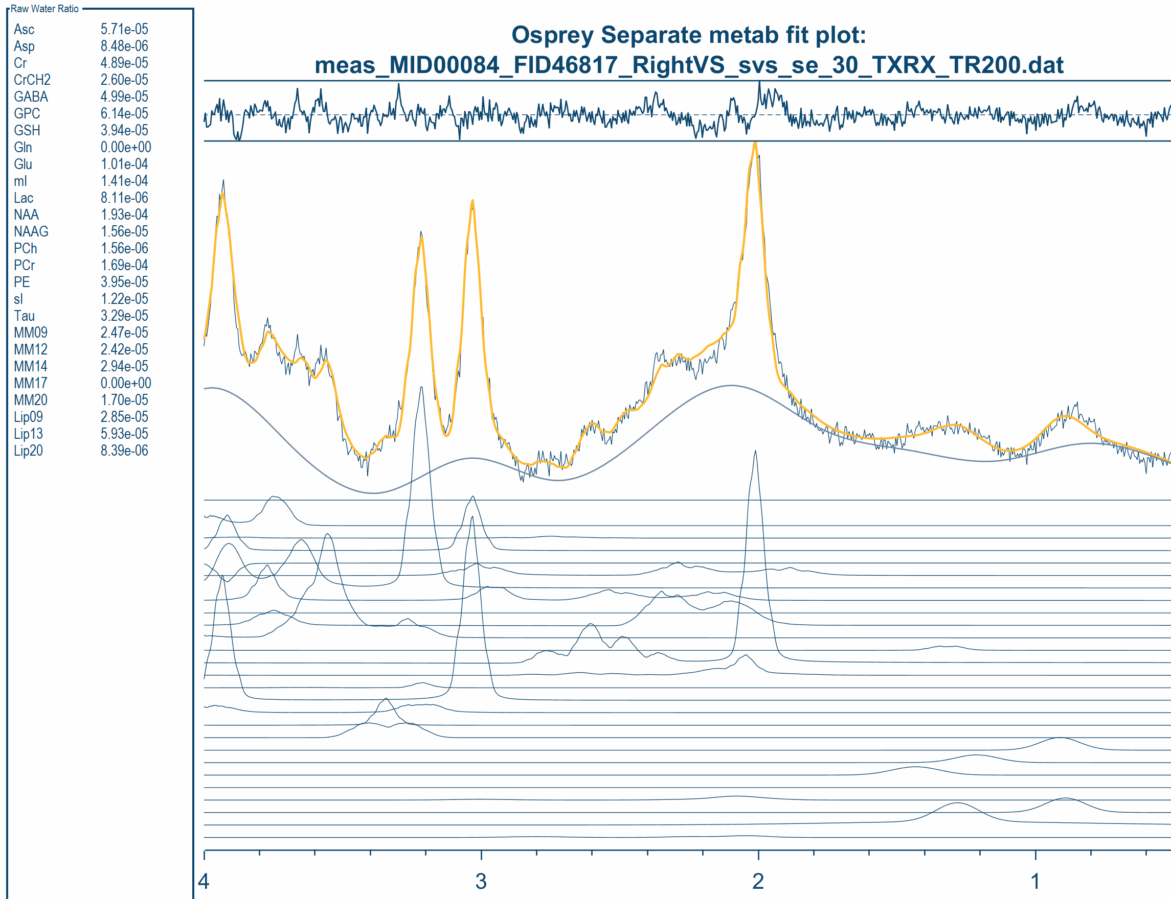
opts.fit.method = ‘LCModel’; % OPTIONS: - ‘Osprey’ (default)
% - ‘LCModel’
% Determine fitting range (in ppm) for the metabolite spectra
opts.fit.range = [0.5 4]; % [ppm] Default: [0.5 4]
%%% ----- OSPREY FITTING OPTIONS -----
% Choose the fitting style for difference-edited datasets (MEGA, HERMES, HERCULES)
% (only available for the Osprey fitting method)
opts.fit.style = ‘Separate’; % OPTIONS: - ‘Separate’ (default) - will fit DIFF and OFF separately
% - ‘Concatenated’ - will fit DIFF and SUM simultaneously)
% Determine fitting range (in ppm) for water spectra
opts.fit.rangeWater = [2.0 7.4]; % [ppm] Default: [2.0 7.4]
% Determine the baseline knot spacing (in ppm) for the metabolite spectra
opts.fit.bLineKnotSpace = 0.4; % [ppm] Default: 0.4.
% Add macromolecule and lipid basis functions to the fit?
opts.fit.fitMM = 1; % OPTIONS: - 0 (no)
% - 1 (yes, default)
% Optional: Deface the strucutral images in the Coreg/Seg figures for HIPAA
% compliance
opts.img.deface = 1;
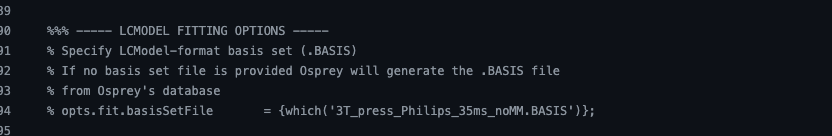
%%% ----- LCMODEL FITTING OPTIONS -----
% Specify LCModel-format basis set (.BASIS)
% If no basis set file is provided Osprey will generate the .BASIS file
% from Osprey’s database
opts.fit.basisSetFile = ‘/Users/otherminds/Desktop/test_MRS/LCM_basis_39.BASIS’;
% The following lines perform an automated set-up of the jobFile which
% takes advatage of the BIDS foramt. If you are not using BIDS (highly
% recommended) you can look at the definitions below the loop to see how to
% set up direct path links to your data.
% Specify LCModel-type control file (.CONTROL)
% This is optional: If you leave this field blank, Osprey will create a
% minimum control file for you.
% opts.fit.controlFile = ‘’;
%%%%%%%%%%%%%%%%%%%%%%%%%%%%%%%%%%%%%%%%%%%%%%%%%%%%%
%%%%%%%%%%%%%%%%%%%%%%%%%%%%%%%%%%%%%%%%%%%%%%%%%%%%%%%
%%% 3. SPECIFY MRS DATA AND STRUCTURAL IMAGING FILES %%
% When using single-average Siemens RDA or DICOM files, specify their
% folders instead of single files!
% Clear existing files
clear files files_ref files_w files_nii files_mm
% Data folder in BIDS format
% The filparts(which()) comment is needed to find the data on your machine. If you set
% up the jobFile for your own data you can set a direct path to your data
% folder e.g., data_folder = /Volumes/MyProject/data/’
data_folder = ‘/Users/otherminds/Desktop/test_MRS/TE39’;
% The following lines perform an automated set-up of the jobFile which
% takes advatage of the BIDS foramt. If you are not using BIDS (highly
% recommended) you can look at the definitions below the loop to see how to
% set up direct path links to your data.
subs = dir(data_folder);
subs(1:2) = ;
subs = subs([subs.isdir]);
subs = subs(contains({subs.name},‘sub’));
counter = 1;
for kk = 1:length(subs)
    % Specify metabolite data
    % (MANDATORY)
    dir_metabolite    = dir([subs(kk).folder filesep subs(kk).name filesep 'mrs' filesep subs(kk).name '_press_act' filesep '*.SDAT']);
    files(counter)      = {[dir_metabolite(end).folder filesep dir_metabolite(end).name]};

    % Specify water reference data for eddy-current correction (same sequence as metabolite data!)
    % (OPTIONAL)
    % Leave empty for GE P-files (.7) - these include water reference data by
    % default.
    dir_ref    = dir([subs(kk).folder filesep subs(kk).name filesep 'mrs' filesep subs(kk).name '_press_ref' filesep '*.SDAT']);
    files_ref(counter)  = {[dir_ref(end).folder filesep dir_ref(end).name]};

    % Specify water data for quantification (e.g. short-TE water scan)
    % (OPTIONAL)
    files_w     = {};

    % Specify metabolite-nulled data for quantification
    % (OPTIONAL)
    files_mm     = {};

   % Specify T1-weighted structural imaging data
    % (OPTIONAL)
    % Link to single NIfTI (*.nii) files for Siemens and Philips data
    % Link to DICOM (*.dcm) folders for GE data
    files_nii(counter)  = {[subs(kk).folder filesep subs(kk).name filesep 'anat' filesep subs(kk).name '_run-01_T1_MPRAGE.nii.gz']};


    % External segmentation results
    % (OPTIONAL)
    % Link to NIfTI (*.nii or *.nii.gz) files with segmentation results
    % Add supply gray matter, white matter, and CSF as 1 x 3 cell within a
    % cell array  or a single 4D file in the same order supplied as 1 x 1 cell;
% files_seg(counter) = {{[sess(ll).folder filesep sess(ll).name filesep ‘anat’ filesep subs(kk).name filesep ‘c1’ sess(ll).name ‘_T1w.nii.gz’],…
% [sess(ll).folder filesep sess(ll).name filesep ‘anat’ filesep subs(kk).name filesep ‘c2’ sess(ll).name ‘_T1w.nii.gz’],…
% [sess(ll).folder filesep sess(ll).name filesep ‘anat’ filesep subs(kk).name filesep ‘c3’ sess(ll).name ‘_T1w.nii.gz’]}};
% files_seg(counter) = {{[sess(ll).folder filesep sess(ll).name filesep ‘anat’ filesep subs(kk).name filesep ‘4D’ sess(ll).name ‘_T1w.nii.gz’]}};
counter = counter + 1;
end
%%%%%%%%%%%%%%%%%%%%%%%%%%%%%%%%%%%%%%%%%%%%%%%%%%%%%%
%%% 4. SPECIFY STAT FILE %%%
% Supply location of a csv file, which contains possible correlation
% measures and group variables. Each column must start with the name of the
% measure. For the grouping variable use ‘group’ and numbers between 1 and
% the number of included groups. If no group is supplied the data will be
% treated as one group. (You can always use the direct path)
file_stat = ‘’;
%%%%%%%%%%%%%%%%%%%%%%%%%%%%%%%
%%% 5. SPECIFY OUTPUT FOLDER %%
% The Osprey data container will be saved as a *.mat file in the output
% folder that you specify below. In addition, any exported files (for use
% with jMRUI, TARQUIN, or LCModel) will be saved in sub-folders.
% Specify output folder (you can always use the direct path)
% (MANDATORY)
outputFolder = fullfile(data_folder, ‘derivatives’);
%%%%%%%%%%%%%%%%%%%%%%%%%%%%%%%
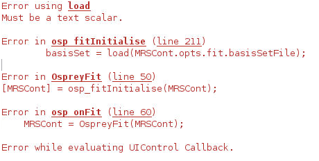
and the errors are:
Brace indexing is not supported for variables of this type.
Error in osp_fitInitialise (line 56)
if ~(isfield(MRSCont.opts.fit,‘basisSetFile’) && ~isempty(MRSCont.opts.fit.basisSetFile) && ~isfolder(MRSCont.opts.fit.basisSetFile{1}))
Error in OspreyFit (line 50)
[MRSCont] = osp_fitInitialise(MRSCont);
Error in osp_onFit (line 36)
MRSCont = OspreyFit(MRSCont);
Error while evaluating UIControl Callback.