Metabolite concentrations calculated by Osprey

[ZeinabEftekhari]

Hi,

I am using Osprey for analyzing my SVS data acquired by STEAM and sLASER at 3T and 7T. I am facing a problem and I do not know why this is happening. I would appreciate it if you could help me.

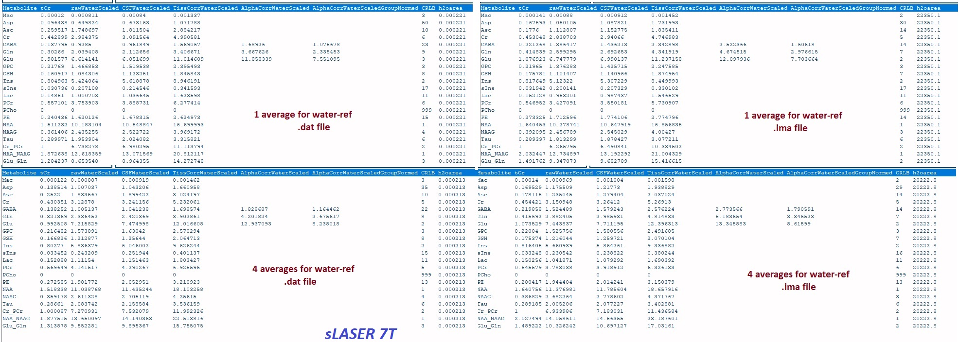
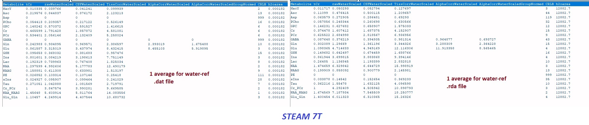
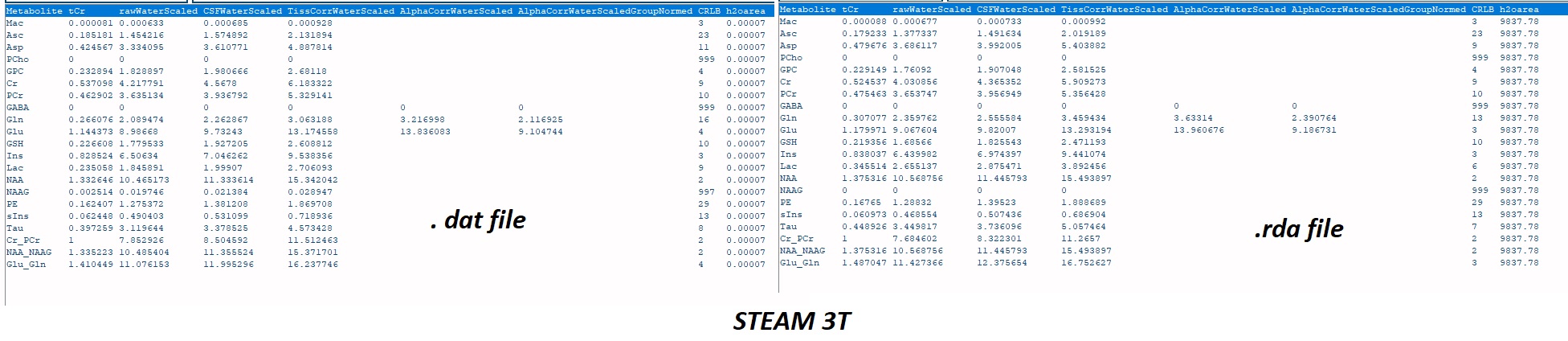
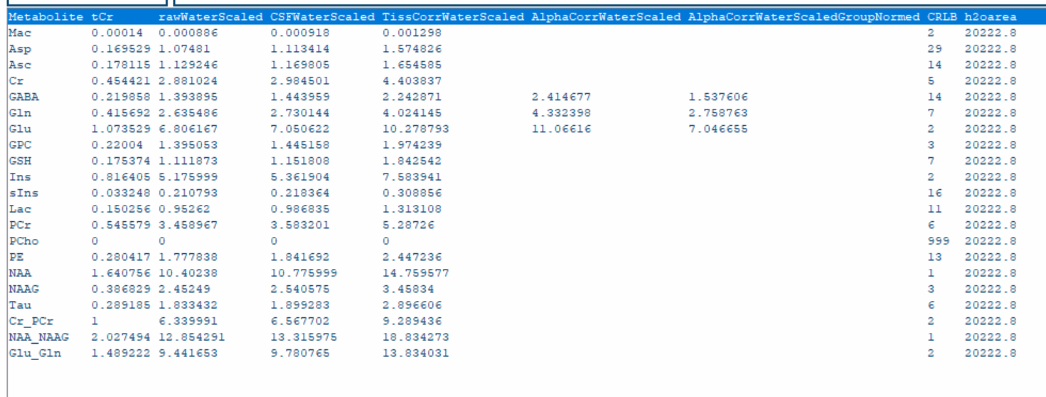
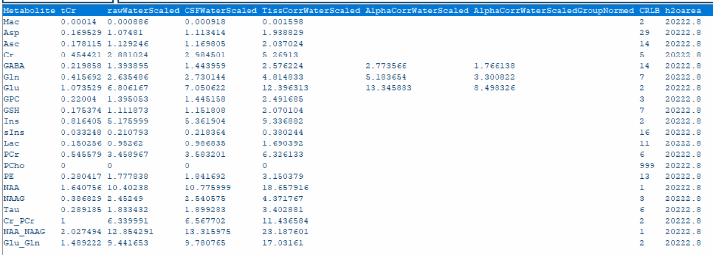
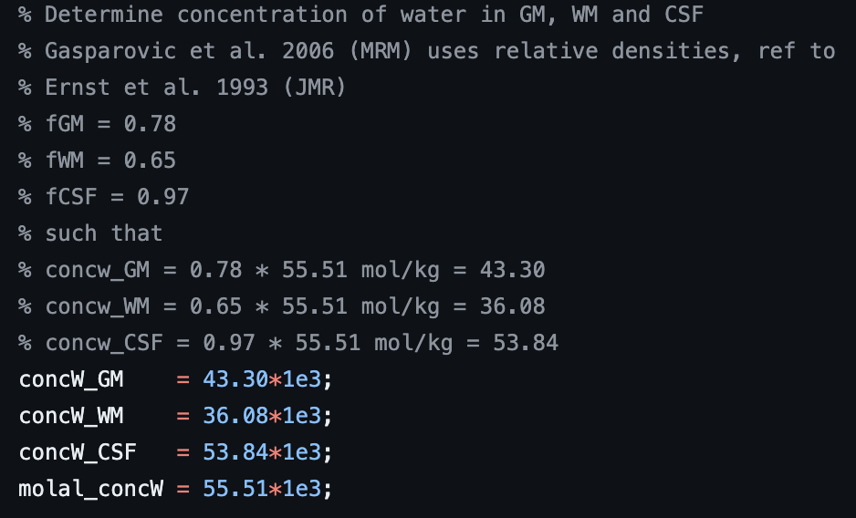
1- All TissCorrected values for both steam and slaser at 3t and 7t are higher than the normal range when I use .ima and .rda formats. I tried with dat format just for steam at 7t, and the values were in the correct range. However, my problem is I do not have the same type of format for all my data.

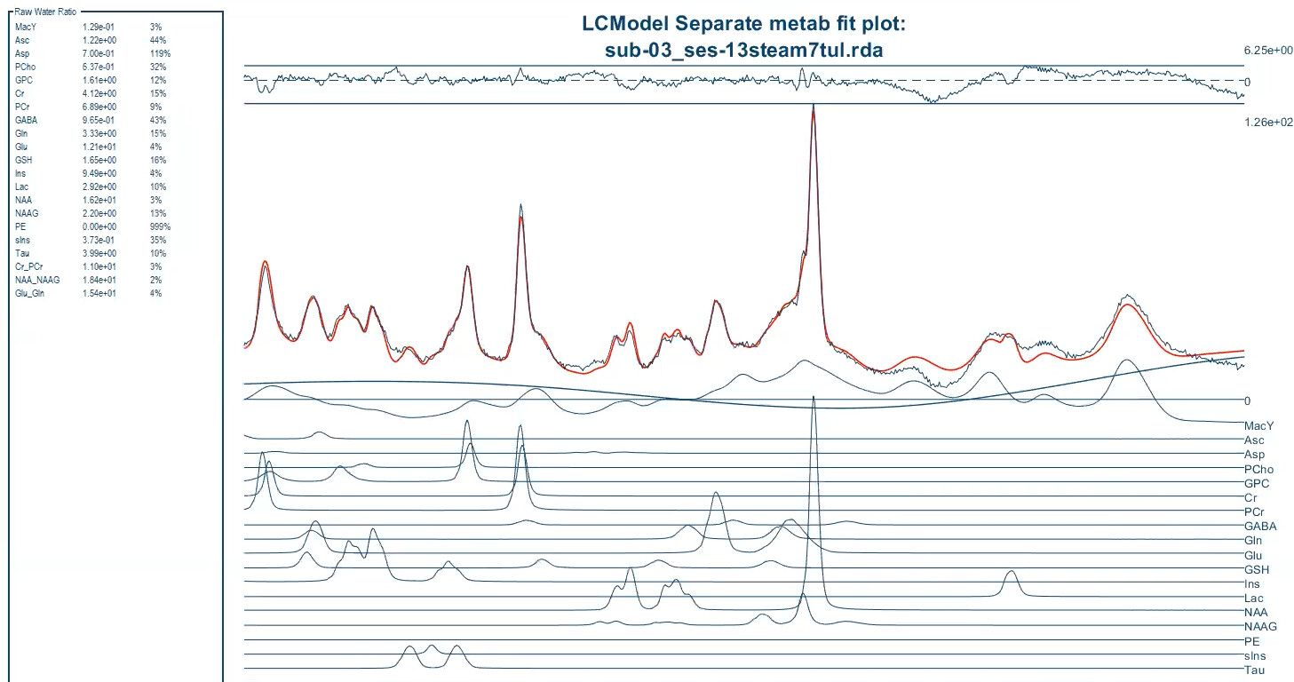
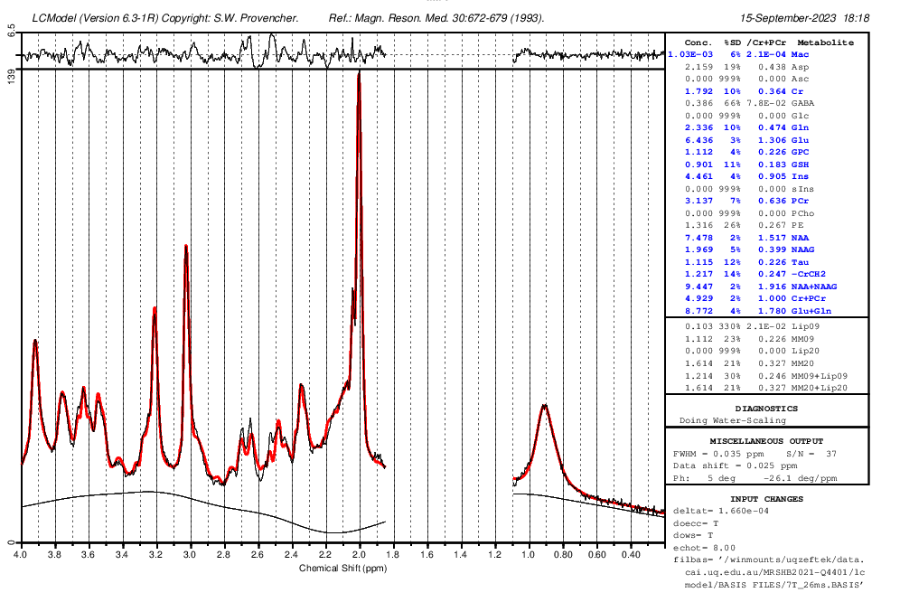
Do you know what should I do so that the values be in the correct range for the .ima and .rda formats? (I put screenshots of quantification tables and a couple of videos to see the quality of fitting and the procedure).

https://filesender.aarnet.edu.au/?s=download&token=41c8b385-333a-43bb-8f13-f373eb693845

2- For STEAM at 3T and 7T, I have dat and rda.
For sLASER at 3T and 7T, I have .ima and rda. All 4 Water reference scans and 32 averages for metabolite data were saved in one dat file for each sLASER, and I do not know how can I separate them. Also, I want to know if it is possible to extract the first 16 averages out of 32 from a dat file and save it as a new file?

[ZeinabEftekhari]

Hi again,

I figured out how to split the dat file for sLASER, and able to analyse the slaser with dat format. However, still the metabolite concentrations for TissueCorrected are overestimated and out of their normal range. It appears that regardless of the format I use, the values remain incorrect, despite the data quality and fitting being satisfactory.

Additionally, I’ve observed that the raw-water values for STEAM at 7T are lower compared to sLASER. This pattern is consistent across all 10 subjects in my scans. But not at 3T. They are roughly similar.

I’ve attached screenshots from the quantification tables for sLASER and STEAM, utilizing various formats.

For sLASER, I had 4 averages for water-ref. I analysed both using all 4 averages and once using one average.

[hraum]

Hi Zeinab,
the difference between rawWaterScaled/CSFWaterScaled and TissCorrWaterScaled is very suprising. When I look into OspreyQuantify.m, the main difference between CSFWaterScaled and TissCorrWaterScaled is that for CSFWaterScaled the water concentration was assumed to be the same for white matter and we have mean relaxation times for T1 and T2. For these factors in TissCorrWaterScaled, tissue fractions were considered. Maybe it’s easier to look at the 7T data, because the CSF fraction looks very small and we can ignore them.
For CSFWaterScaled we have for water:
water concentration = 55600 (pure water)0.65 (water visibility for wm) = 36140 mmol/L
T1_Water = 1.675;
T2_Water = 0.0525;
For TissCorrWaterScaled we have for water (ignore CSF):
water concentratration = 43300 (GM) and 36080 (WM)
T1_water = 2.130 (GM) and 1.220 (WM)
T2_water = 0.055 (GM) and 0.050 (WM).
The difference of the used relaxation times is to similar to explain your effects, I think.
But when we have a closer look to the formulas, CSFWaterScaled is scaled by pure water concentrationwater visibility. For TissCorrWaterScaled, I don’t see this factor (e.g. set molal_fWM=1, only molal_concW=55510 is left).
This can explain that you have about 50% higher concentrations with tissue correction. Maybe @admin can help why these differences in the formulas exist.

Best, Heiner

[ZeinabEftekhari]

Hi Hiener,

Thanks a lot for your response and explanation. I believe I may have identified another factor contributing to the overestimation of my data. Please correct me if I’m mistaken.
I am using Dinesh sLASER sequence, it has 3 TEs: TE1=7; TE2=10;TE3=9 and the combination of these are the actual echo time that I am using (26 ms). In Osprey header we can only see TE1 (below is the screenshot), I believe it may only consider this TE for adjusting the Echo time and based on this do the quantifications:

In this script "OspreyQuantify.m, line 246, is for getting the echo time, I manually changed “MRSCont.processed.metab{kk}.te” to 26 ms, and here is the value after and before this change:

I couldnot find anywhere else in the codes except the one I mentioned for getting the TE, if I have to change it from somewhere else, please let me know. How about line 594 and 595?

After changing TE to 26ms(In the header TE is still 7):

Before changing:

@Helge I’d like to hear your thoughts on this issue. Your assistance and suggestions would be greatly valued.

[hraum]

Hi Zeinab,
you’re absolutely right. This is also a problem here. At the beginning, I was also thinking about it. But normally, that should have an effect on both, RawWaterScaled/CSFWaterScaled and TissCorWaterScaled. So I’m wondering, why your results didn’t change for CSFWaterScaled, only for TissCorWaterScaled.
You also have to take into account that waterTE should probably be corrected. When you set your TE values correctly in line 246-247, you needn’t change line 594-595.
And normally the metabolite concentration should be proportional to 1/exp(-TE/T2_Metab). When you increase TE in your calculations, the estimated concentrations should also increase, or not?
Because of that and the fact that rawWaterScaled/CSFWaterScaled isn’t changing, I’m afraid that we overlooked something. Maybe you can correct TE in your data.

Best,
Heiner

[Helge]

Hi @ZeinabEftekhari,

sorry for the delay. There are several things to unpack for your dataset.

OspreyQuantify issues: You are actually right that there is something off with the quantification module. Apparently, the code converted the TE/TR values from ms to seconds in lines 246-247, but divided them by 1000 again in the quantH2O function (which produces the input for the CSF-corrected estimates). The values were therefore extremely small and changing the TE values had almost no effect on the quantification. I have just pushed a fix to GitHub to resolve this. It is fine to change the TE/TR values in lines 246-247 only. However, I’d would be better to resolve this by correctly parsing the header information during the OspreyLoad module. Could you take a look at this yourself and see if you can find the correct TE values from the header or share the data with me?

OspreyFit: I had a quick flick through your data because I was worried by the variance in the tNAA estimates. It seems like LCModel has problems with the scaling/quantification of the measured MM basis set you are using. In some cases, it is almost zero and the spline baseline is doing the only work for the macromolecules leading to very high metabolite estimates. This was mainly the case for subjects with lipid contamination. This definitely needs fixing. There are several possible ways to do this:

1. Scale the MM basis function to have a similar scale as the rest of the basis set
2. Exclude the frequency region between 1.1 and 1.85 ppm using the LCModel GAP settings in the control file
3. Use Gaussian parameterized MM basis functions instead

Let me know how this works out.

You should also do a bit of quality control where you look for lipid contamination or out-of-volume signals before using the estimates.

@hraum Thank you for jumping in! About the differences in the formulas. For the TissueCorrected estimates, we are applying the water visibility factors in the very beginning (see pircture). Therefore, molal_fWM = 1 is similar to 55510 * 0.65.

Best,
Helge

[hraum]

Hi @Helge,
Thanks for your answer. I’m still not understanding how you take the water visibility factors into account. Indeed, they are included in concW_GM, concW_WM… But I see these concentrations only in calculations for the molal fraction (line 713-715). In the calculations for TissCorrWaterScaled (line 729-733), I just see that molal_concW is included and for molal_fWM = 1 I achieve:
TissCorrWaterScaled{mm,ss}.metab(kk, = (amplMets{mm,ss}.metab(kk, ./ amplWater) .* molal_concW .* (1 - exp(-waterTR/T1w_WM)) * exp(-waterTE/T2w_WM) / ((1 - exp(-metsTR/T1_Metab(kk))) * exp(-metsTE/T2_Metab(kk)));
Am I missing something?

Best,
Heiner

[ZeinabEftekhari]

Hi Helge,

Thank you for your help! It was very helpful.

Regarding OspreyQuanity, I figured out how to adjust TE in osp_LoadDICOM and osp_LoadTwix. Also in OspreyQuality.m when I removed lines 594 and 595, it improved CSFWaterScaled results, which are now closer to the right range.

As for OspreyFit, I understand that you mentioned in the data with lipid contaminations the metabolite concentrations are higher and you found out because of tNAA values fluctuations. However, I’m not clear on the exact reason. For instance, in data with lipid contamination using STEAM, what’s the issue with scaling MM?

I’m using the basis set provided by Dinesh and Gosia, which includes measured macromolecules. In the control file, I set NSIMUL=0 and dkntmn=5, and I removed the chomit = ‘Mac’ command from the default Osprey control file. Because I didn’t create the basis set myself, I need help with the first and third solutions you suggested. Can you please explain how to do them and clarify the difference between these three solution? If there’s no difference, I attempted the second solution by using these commands: ppmgap(1,1) = 1.85 and ppmgap(2,1) = 1.1. However, I encountered an error in Osprey.

 FATAL ERROR  MYCONT  2.   (Check LCModel Manual).  ************************************************************************ 

*** FATAL ERROR MYCONT 2
This error occurred before the plot could be produced.
See the Diagnostics list in the LCModel Manual. ***

I tried the same command with LCModel, and it worked successfully.

If I implement the second solution for my data, given that we’re disregarding macromolecule (MM) concentrations within this gap, could this approach potentially impact the accuracy of the overall metabolite quantification?

Best,
Zeinab

[richardedden]

Hi @hraum and @ZeinabEftekhari,
I’ve just been reviewing these equations with @Helge and trying to remember when we have gone around this whole discussion previously.

A lot of the confusion here arises from the units… my instinct (as a chemist originally) is to measure concentration as a molar quantity (moles per volume), whereas the in vivo community often use a molal quantity (moles per mass of solute). This distinction makes sense in terms of context (pure homogeneous solution vs. murky biological sample).

Within the Osprey equations, the different options have been inherited from different sources, and the CSFWaterScaled is a “molar-family” quantity. At some point, as a result of some vigorous reviewing on our manuscripts, we adopted the Gasparovic [Magnetic Resonance in Medicine 55:1219–1226 (2006)] convention which is “molal-family”. This is the case for the TissCorrWaterScaled quantity in Osprey.

The point that made it all come together for me was that MOLAL units are “moles per kg of MR-visible solute”. So if I have a 10 mmol/dm^3 molar concentration, with a solute visibility fraction of 0.65, I would expect to get a 15 mmol/kg molal concentration.

I may just be reiterating things that you have worked out yourselves above, but I thought it might be worth weighing in.

LCModel is in the molar family, but community consensus is not to stop at LCmodel output, but apply further corrections (which often convert the numbers into molal-family). We could do better as a community in discussing these points (and I think the discussion of units in the consensus terminology ignores/misses this question). The quantification consensus (doi: 10.1002/nbm.4257.) does get into it a bit deeper.

[Helge]

Hi @ZeinabEftekhari,

Not sure if I can follow which line you have removed (seems like the lines that define the pure water concentrations in mmol/L and the water visibility. If you do this you won’t have molar concentration for the WaterScaled and the CSFWaterScaled estimates anymore.

About the tNAA fluctuations, the spectrum you posted has a reasonable fit, however, there were datasets where LCModel estimated almost zero macromolecules and everything was modeled with the spline baseline (I have actually deleted your data again so I can’t tell you which dataset it was). You should look into these and how they improve with the gap parameter or the Gaussian MMs.

The second LCModel output looks fine apart from the fact that you are now using measured macromolecules and Gaussian ones! You should only include either one of those.

Best,
Helge

[hraum]

Hi @richardedden,
Thanks a lot for your answer. Indeed, it is really confusing because of the units. Maybe I am missing something, but both on the manual (Chapter 5 Osprey GUI tutorial | Osprey Documentation) and the puplication (10.1016/j.jneumeth.2020.108827), the units are not clearly obvious of CSFWaterScaled and TissCorrWaterScaled. For the latter, I only see that " Osprey reports water-scaled metabolite estimates according to Equation 5, analogous to the LCModel water scaling procedure" and " Osprey derives fully tissue-and-relaxation-corrected molal concentration estimates according to the Gasparovic method".
Maybe Osprey can highlight this more because normally, I would assume as user that both columns would have the same unit.
In this context, another question: in LCModel, mM stands for “mmol per Kg wet weight” and actual mM should be multiplied by 1.04 (see LCModel manual). When I use the algorithm from “Osprey” or from “LCModel” is this factor taken into account?

Best,
Heiner

[richardedden]

Thank you for highlighting this.

I have to admit that, until we started this conversation, I was not aware that the calculations were different in their molaXity. (Maybe now is not the best moment to invent a new term for molarity/molality). @admin and @Helge may have, but for me, the units have never been particularly interesting… Indeed, I have tended always to fudge toward using ‘i.u.’ deliberately to avoid questions of true absolute quantification (although obviously the equations themselves have an inherent dimensionality that I can’t really escape).

I have never heard of the 1.04 factor before, but might look into it… I have NEVER seen mM used as a shorthand for molality, only molarity. I thought LCModel was dealing in molarities, but maybe there I am also wrong… I started writing my own code because I never liked LCModel, so i haven’t dug deeply. @admin has much more so.

@Helge just told me it corrects for ‘gravity’ - I guess the density difference between tissue and water. i i think in our calculations we wouldn’t need something like that because we already include MR-visibile water concentrations (in mol per volume).

Maybe LCModel concentrations are neither molality not molarity, or a molality referenced to total water weight not the MR-visible weight, or…? Again, I am not the LCModel whisperer.

[hraum]

Thanks for your answer. Indeed, LCModel has it’s “own” units.
“Concentrations should be labeled “mmol per Kg wet weight”. We use the shorter (incorrect)
abbreviation mM. The actual mM is the mmol per Kg wet weight multiplied
by the specific gravity of the tissue, typically 1.04 in brain.” (from manual)
But all in all, it is comparable with molarity although it is per kilogram, except the factor 1.04. For the calculations in Osprey, the factor 1.04 should be only interesting when the LCModel algorithm is used for fitting that you have the correct unit mM and can compare it with your own algorithm.

Best,
Heiner

[Jude]

Hi Zeinab,

I was deeply inspired by your question. I would like to ask how you saw CRLB bounds when quantifying the results of your data. The data I tried to quantify myself will not appear CRLB. And how to solve the problem of reading only TE1 in the end. Thank you. looking forward to your reply

[admin]

In the current version, CRLB will only show up if you model the data with the internal LCModel fitting option.

The TE1 problem should have been fixed with the January 22 commit to the develop branch - please pull code from there instead of the release version.